Getting Started with Data Load Rules in Oracle PBCS

A quick look at what they are, how they work, and why they matter.

Data load rules are associated with something called “integrations”. This scares some consultants off, especially those who have never touched them and may psychologically feel like this is a never ending black hole that you just want to avoid at all costs. It’s the fear of the unknown. I know how this feels because I too have been there.

If that’s how integrations make you feel, this blog on integrations is for you.

This whistle stop tour should give you some confidence in integrations, how they work in principle and replace some of that hidden anxiety with curiosity.

What is a data load rule?

A data load rule (”DLR” for short) is an integration which is set up within Oracle PBCS for digesting data which can come from a particular “source”. A source could be a file, or another solution which holds the data to be brought in such as an ERP solution or an external database.

Data is like a bowl of cereal. When we eat cereal, it’s the same concept as loading data into PBCS (the stomach), we’re simply getting it into the system.

But just swallowing cereal isn’t enough. Your body needs to digest it, break it down, and convert it into something useful.

In the same way, Oracle PBCS needs the right Data Load Rule (DLR) setup so it can interpret the incoming data, transform it, and put it in the correct place inside the application.

Data sources for data load rules explained

These are some of the common source types which commonly occur in most EPM implementations:

1. File Based - This is a separated values file (csv, txt or an xlsx excel file).

2. Oracle ERP Cloud - Certain Oracle ERP modules can be directly integrated with the EPM application at hand, such as the typical general ledger.

3. Business intelligence Publisher (BIP) Reports - These are custom built reports in Fusion ERP which are built using the SQL coding language.

(Note: not all ERPs can be integrated directly. Please ensure to review Oracle documentation to ensure your architecture is possible)

How do I set up a data load rule?

You can create data load rules from two places at present in Oracle PBCS, the old data management which can be found by clicking on the three horizontal lines in the top left of the application called a “burger” menu, or the newer “data integration”.

I’ll be highlighting the newer data management which is called “Data Integration” found within “Data Exchange”.

1. Go to Application —> Data Exchange —> Data Integration —> Click the “+” button, and select “Integration”.

   

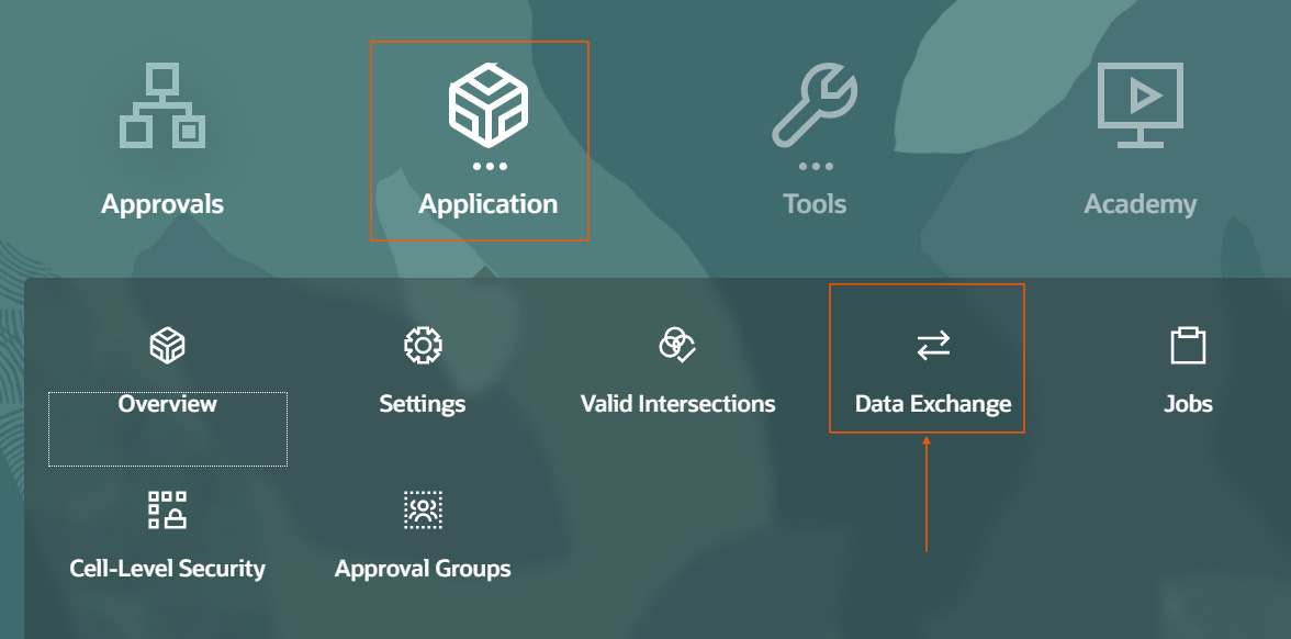
2. The tab to the left called “Data Integration” is where you need to be for creating data load rules.

   

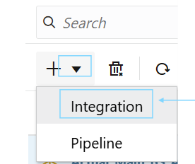
3. To create a Data Load Rule, click the “+” icon and select “integration”.

   

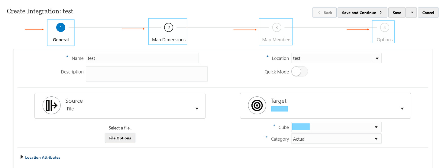
4. This will bring the following menu below. Creating a Data Load Rule has 4 main sections, these are highlighted in the BLUE boxes further down.

   1. General

   2. Map Dimensions

   3. Map Members

   4. Options

      

An overall summary can be found below of each section:

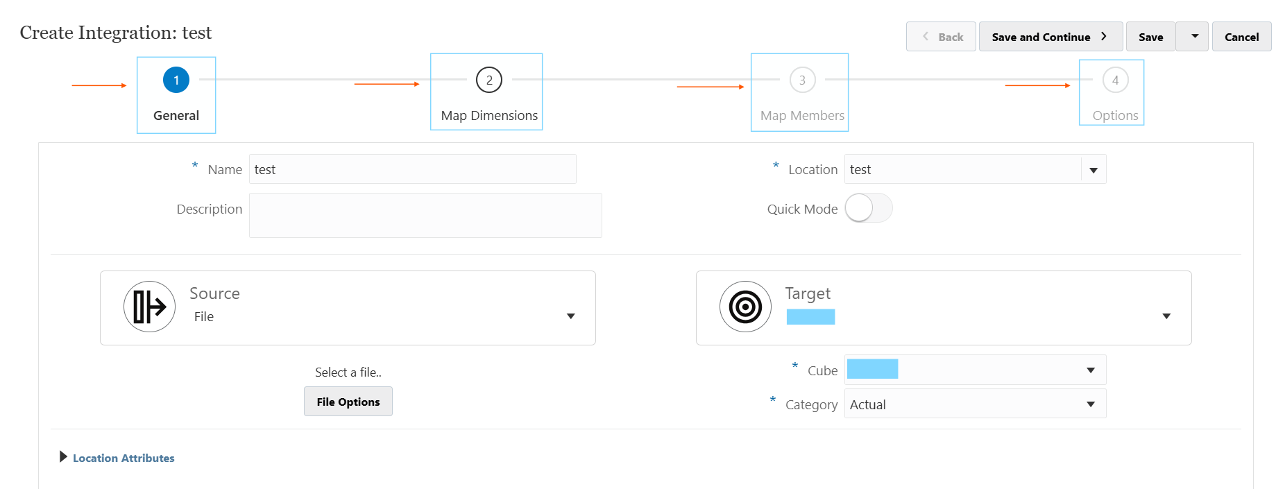
1. General

   In the first tab of a Data Load Rule, you define the foundational mapping between where the data is coming from and where it will be loaded to.

   1. Location represents the combination of a specific source system and import format, along with the associated mappings and load rules.

   2. Source is where the data is coming from. In the image above, a file is selected as the source.

   3. Target is the EPM target application. It can be PBCS, FCCS etc.

   4. Cube is the target plan type, which is essentially the cube where the data is going to load into.

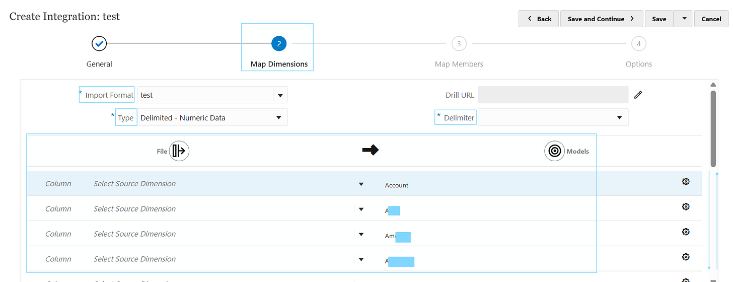
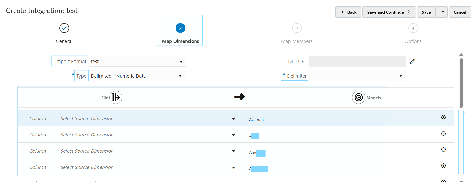
2. Map Dimensions

Remember, Oracle EPM applications are multi dimensional databases, so think of a rubik’s cube with multiple sides when going through this.

1. Input format is the set up of the entire sub tab, which is the name of the format being defined for the DLR.

   1. It’s a good practice to have a unique input format per data load rule. Because if you share them across DLRs and one changes in the future, it’s going to have a knock on affect on other DLRs and essentially break them…this can get messy very quickly and create serious panic in a business, so avoid this.

2. Type is how the file is to be treated. There are numerous types which I’ll cover separately but the example of Delimited - Numeric data means there is going to be one amount column, along with multiple descriptor (or intersection) columns.

3. Delimiter refers to the source file being used. So, if it’s a comma separated values file with a semi colon delimiter, the delimiter will be a semi colon “;”. You can see the preview when you upload the file and choose the “next” button in “file options”.

4. The bottom half is where all the source mappings from the file are lined up with the target intersections of the target cube.

   1. The column fields are where you’d put the column number of the field being mapped to the target dimension on the right side.

      1. e.g. column 3 of the file called Account, maps to the Account dimension. So, Column = 3, Select Source Dimension = “Account” and the target dimension = Account.

      2. You can do transformations of values coming in too, so if it needs a prefix, a suffix or a certain condition to treat the data, you can do all of that in here. So it’s not always necessary to do it in the source file as often it’s far easier to do directly in the data load rule set-up.

         

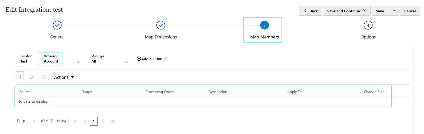
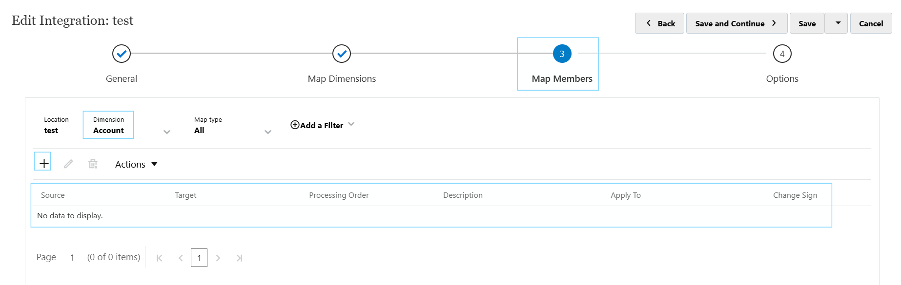
5. Map members

   1. This is where the actual data values are mapped from the source file to the target dimensions. You can do various types of mappings, not just 1-1, but multi dimensional combining more than one dimension based on a condition, 1 to many etc.

   2. In each dimension, there are mappings which can be added with the “+”. It’s important to add “like” mappings because the data which matches the target you want it to slot straight into the target cube without any need to add mappings.

      1. * Source TO * Target is a like-for-like mapping. So for instance, it will load everything without mappings when this is present, assuming the values align with the target values in PBCS.

      2. For any mappings where the source value and target values are not the same, a specific mapping must be added.

         

6. Options

   1. Category selects the scenario you’re loading into (e.g. Actuals).

   2. Period Mapping Type chooses how periods are treated from the source and translated into the target application.

   3. Calendar is the reference to the “explicit” period mapping types list, which allows you to select defined period mappings specifically for the data load rule.

   4. Directory defines the folder where source files are expected for file‑based integrations

   5. File Name is the unique name of the source file being loaded.

   6. Batch Size controls how many records are processed per batch during export.

   7. Drill Region enables the automatic drill‑through of regions in the application.

   8. Clear Region lets you specify exactly which slice of the target to clear when using Replace mode, including:

      1. Dimensions to include, member functions, lists, or “derive from data” and optional filter expressions.

How do I run the data load rule after it’s set up?

1. To run a data load rule, you go to the data load rules screen, and hit the play button to the right for the specific data load rule you want to run.

   

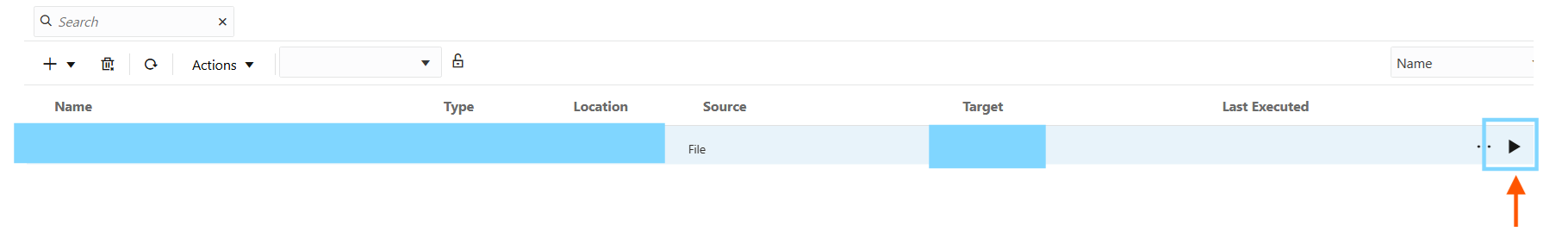
1. When you “run” a data load rule, you are prompted with the below parameters.

   

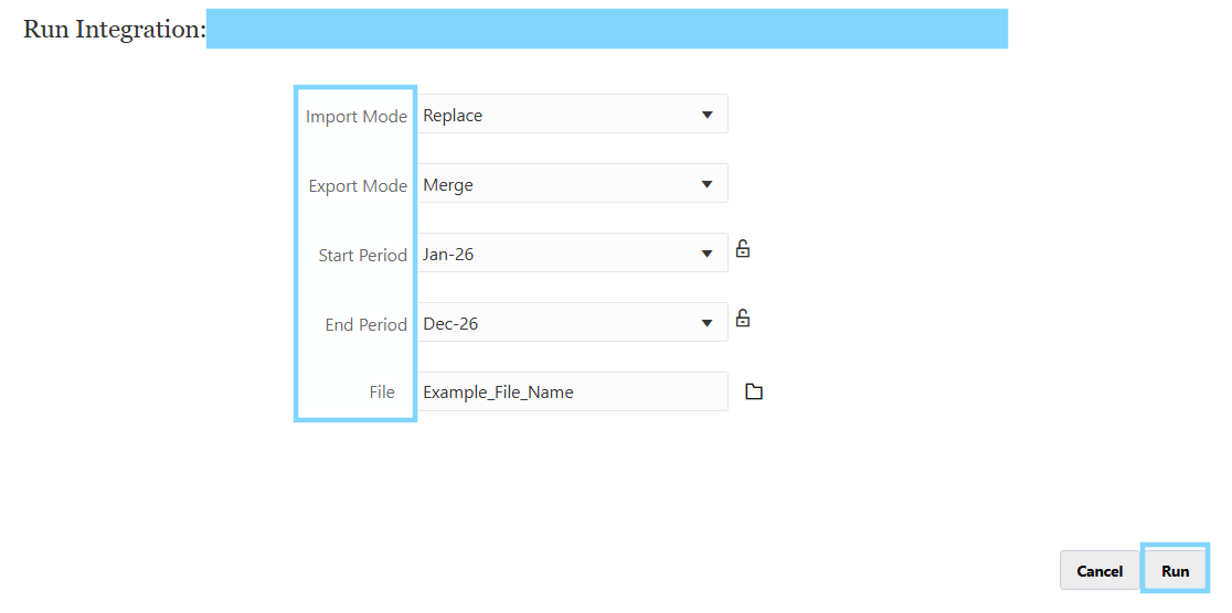
2. Import Mode is the way the data loads into the workbench in the application, we call this the staging area where you can preview how the data comes in before it is pushed into the application. It’s easy to spot a problem in the workbench because it gives a preview of the source and target columns side by side.

3. Export mode is when the data is loaded from the workbench, into the target application.

4. Start period & End period are the start and end periods for the range of the data load rule to cycle through.

   1. Usually this is yearly (unless in a pipeline, which is something more advanced where you can cycle through multiple loads in ONE LOAD, how efficient! I’ll cover this in a future blog)

5. File name is the selection of the file to use to load as the source file. Or it would automatically be picked up if it’s connecting to a cloud source system like ERP Fusion.

Data is the foundation of any software application for pretty much anything in life. Incorrect data means any outputs which used for decision making are going to be fundamentally incorrect, so it’s an underappreciated area which I hope to shine more light on in the coming weeks as I delve deeper on this misunderstood topic.

Integrations are complex, and explaining it is even more complicated, but once you get your head around the data transformation process, it’s something exceptional.

As always, I appreciate your time to read, I hope you managed to keep up (if you need any clarity on any of the bits covered just send a message below and I’d be happy to explain further) - I’ll catch you in the next one!